Writing your own genRhs.py
The functions called in the genRhs.py are documented in the API reference section. However, this section aims to elucidate the order and reasoning behinds the various steps when setting up the Partial Differential Equations (PDEs) system to be solved together with Boundary Conditions (BCs) and specifying numerical parameters associated to the automatic discretisation of derivative operators. A section aiming at describing how loop-distribution and -fusion can conveniently be done without digging into the Fortran layer is also provided.
How to generate the discretised equations
genRhs.py is the user-level module that specifies the system of equations to be marched in time. For convenience, this process is often divided into two steps: 1) the PDEs and BCs specifications through a series of dictionaries and lists, and 2) the Fortran source code generation through appropriate calls to genKer.py user-level functions.
Assume that ones want to march in time the 2D compressible Euler equations given by:
Setting equations in equations.py
PDEs and BCs specifications are typically done in a separate file, hereafter named equations.py. This file should contain the set of PDEs provided through dictionaries (see below) and a series of specific lists needed by dNami. The first parameter to be put in equations.py is the number of spatial dimensions:
dim = 2 # can be 1,2 or 3
Dictionaries of equations
dNami does not contain any preset symbols or limited forms of PDEs. It is the user responsibility to declare the list of symbols needed to write the PDEs that will be marched in time and the corresponding equations. This is done through the varname dictionary (needed by the framework):
varname  = {'rho' : 1,
            'u'   : 2,
            'v'   : 3,
            'et'  : 4,
            }
The order set with the indexes in varname corresponds to data location in memory. Variables solved in the left-hand side are specified in varsolved.
varsolved = ['rho','u','v','et']
Setting RHS equations is done through a dictionary of the form
{'Variable Name': 'Pseudo-Code Eqns'}
The Variable Name must match one of the varname keys. Pseudo-Code Eqns refers to symbolic expressions using varname keys or Fortran compatible syntax (Fortran internal functions are allowed here).
Warning
Although dNami marches in time systems of the form:
\[\dfrac{\partial \textbf{q} }{\partial t} = f\left( \textbf{q} \right)\]
The 'Pseudo-Code Eqns' fed to the code generation step and referred throughout this documentation as ‘RHS’ must be equal to \(-f(\textbf{q})\) i.e.:
{'Variable Name': 'Pseudo-Code Eqns for -f(q)'}
For the x derivative of the RHS in the 2D Euler equations we would write:
divFx = {'rho' : ' [ rho*u           ]_1x ',
         'u'   : ' [ rho*u*u + p     ]_1x ',
         'v'   : ' [ rho*v*u         ]_1x ',
         'et'  : ' [ (rho*et + p )*u ]_1x ',
        }
In this expression the pressure is introduced through a new symbol, 'p', not defined in varname. Two possibilities are offered by dNami in such cases. The first one is to provide an equation that relates 'p' with varname variables, this is done through the varloc dictionary:
varloc = { 'e' : ' (et - 0.5_wp*u*u) ',
           'p' : '       rho*e       ',
         }
dNami will automatically replace any occurrence of 'p' with the corresponding combination of varname variables in all treatment of 'Pseudo-Code Eqns' provided to the kernel (through append_Rhs or genBC).
Another option is to allocate static memory for 'p' and compute 'p' before filling the RHS, where only memory access to that location are done. This is done through the varstored dictionary:
varloc    = {'e' : ' (et - 0.5_wp*u*u) '}
varstored = {'p' : {'symb': 'rho*e', 'ind': 1, 'static': True}
In this example, an equation is provided to compute 'e' from varname and 'p' is stored at the first location of the stored-data memory. For what follows, we will assume that the x and y derivative of the flux function have been grouped in one dictionary divF as :
divF = {'rho' : ' [ rho*u           ]_1x  + [ rho*v           ]_1y ',
        'u'   : ' [ rho*u*u + p     ]_1x  + [ rho*u*v         ]_1y ',
        'v'   : ' [ rho*v*u         ]_1x  + [ rho*v*v + p     ]_1y ',
        'et'  : ' [ (rho*et + p )*u ]_1x  + [ (rho*et + p )*v ]_1y ',
        }
Filling out the genRhs.py: Compulsory steps
The first lines in any genRhs.py will involve importing the necessary code-construction functions from the genKer.py. Then, the working precision of the computation is specified via the wp variable.
from genKer import rhsinfo, genrk3, genrk3update, genFilter, genBC, append_Rhs, genbcsrc
import os

wp = 'float64'
dNami offers the flexibility of using a combination of different numerical schemes as well as a filter with each relying on a stencil size that need not be identical. Fig. 23. illustrates the stencils for a filter that uses 11 points and a finite-difference scheme that uses 5 points.
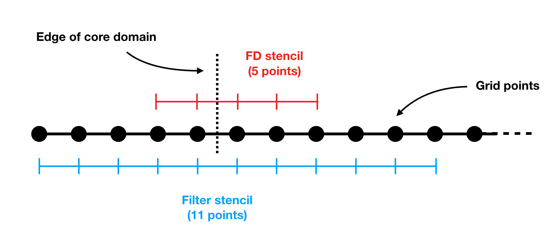
Fig. 23 Two different stencil sizes
To construct the loops over the domain, the genRhs.py requires the user to specify the overall largest number of halo points required to satisfy all the stencil sizes used in the run. In the example of Fig. 23, this would be 5. The hlo_glob variable is used to give this information to the code-generation process:
hlo_glob = 5
Next, the user must initialise the rhs class which is used to store and transfer information from one step to the next:
from genKer import rhs_info
rhs = rhs_info(dim,wp,hlo_glob,incPATH,varsolved,varname,
               consvar=consvar,varstored=varstored,varloc=varloc,
               coefficients=coefficients)
The equations declared in the equations.py are thus stored by the rhs class as well as the number of dimensions, the maximum halo size, etc. This information is used in the following pseudo-code translation steps. Then, the Runge–Kutta time-marching steps are generated with calls to the following functions:
genrk3(      len(varsolved),rhs=rhs)
genrk3update(len(varsolved),rhs=rhs)
Finally, at least one equation must be specified to set the RHS used to march the variables in time, for example:
append_Rhs(divF,5,4,rhsname,vnamesrc_divF,update=False,rhs=rhs,stored=False)
which generates the discretised version of divF using a 5 point, 4th order centered finite difference scheme with rhsname being used to generate code comments and vnamesrc_divF being used to generate intermediate variable names. The update=False argument guarantees that the components of divF are being used to set the RHS rather than be added to existing terms. The stored=False argument determines if the stored variables (see the related Advanced use section below) are computed with the stencil/order given as input to the append_Rhs() function; note that only one call with stored=True is possible, i.e. all stored quantities will be discretised with the same scheme.
This ends the list of compulsory steps when creating a genRhs.py.
Warning
When no boundary conditions are specified in a given direction, the default behaviour assumes that the direction is periodic.
Conservative formulation
Conservation laws in physic can be written in multiple mathematically equivalent forms, yet numerical methods or implementation considerations may dictate specific choices. A classical formulation in continuum mechanics is the so-called divergence form:
where the \(\textbf{q}\) vector takes the form of \(\left[ \rho, \rho \mathrm{var1}, \rho \mathrm{var2},\cdots\right]^{\intercal}\) and the flux tensor \(\textbf{F}\) is made explicit. Conservation of mass may then be ensured exactly with any finite-difference discretisation of the divergence operator, providing that appropriate numerical fluxes are defined based on \(\textbf{F}\) [Vin89]. The divergence form is therefore often referred as conservative formulation in continuum mechanics.
dNami offers the user the possibility of advancing the equations in time using a conservative formulation while minimising data transfer. Note, however, that dNami does not automatically enforce conservativity through appropriate numerical fluxes computation yet. It only generates classical finite-differences of \(\textbf{F}\). In the Euler equations given above, the ‘solved’ variables, which are actually stored in memory, are rho, u, v and et but the quantities advanced in time by the Runge–Kutta scheme are rho, rho*u, rho*v and rho*et, referred to as the conserved variables. In practice, having access to the ‘solved’ variables is useful for setting initial conditions, boundary conditions and outputting information at run time. This requires a transformation between the solved variables and the conserved variables before and after the Runge–Kutta steps. Having access to the solved variables is crucial for efficient computation of the right-hand side of the time-advancement equations as it is more readily expressed as a function of the solved variables rather than the conserved variables. Substitutions of the form (rho*vari)/rho would be necessary and severely detrimental to efficiency if the switch was not performed.
Currently, given a list of solved variables and a variable with the protected name rho e.g.
varsolved = [rho, var1, var2, var3, var4, var5, ..., varN]
the user can choose which variables will be time-advanced in the form rho*varN using the consvar list (note that indexing starts at 1 as this information is passed to the Fortran layer) e.g.
consvar = [3,5,6]
which corresponds to var2, var4 and var5. Note that a mix of equations formulated in a conservative and non-conservative manner can be advanced simultaneously.
Filling out the genRhs.py: Optional steps
The user has access to a number of additional automatic code-generation steps detailed here.
Adding explicit filtering
To add explicit filtering to the computation, the user can call the genFilter function. Currently, the function relies on pre-specified coefficients for a given stencil/order (which can be found at the start of the genKer.py file). For example, the following code block generates code to apply a standard 11 point, 10th order filter to each of the directions (between 1 and 3 depending on dim):
# Generate Filters (if required):
genFilter(11,10,len(varsolved),rhs=rhs)
The user can specify the filter amplitude in the compute.py.
Adding boundary conditions
When non-periodic boundary conditions are enforced, the user must do two things: choose what happens between the core and the boundaries (i.e. those who do not have enough neighbours for the full stencil width) and specify the boundary conditions. These two sets of points are illustrated in Fig. 24.
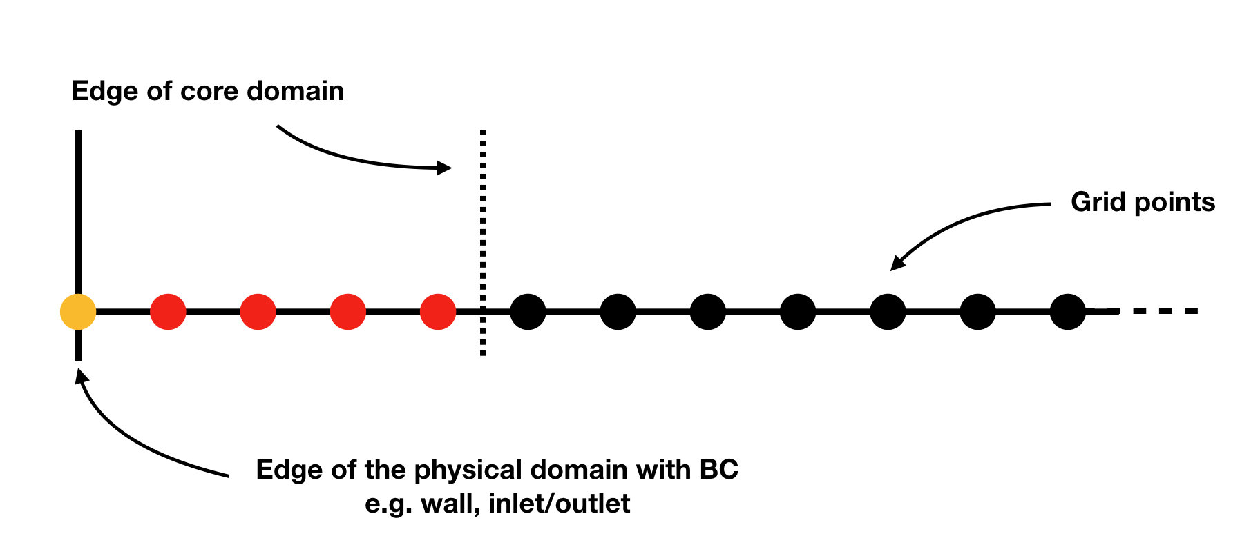
Fig. 24 The two sets of points that must be managed seperately from the core of the domain: the physical boundary points (orange) and the points that do not have enough neighbours for the full stencil width (red)
Both of these cases are dealt with via calls to the genBC() function.
The following code block details the two steps: after calling the append_Rhs() function, a first call to genBC() is made. This performs an automatic stencil and order reduction of the finite-difference schemes and the filter (based on the set of coefficients currently included in dNami) as the boundary is approached. However this does nothing for the actual boundary point (shown in orange in Fig. 24). That point is handled by additional calls to genBC() for each boundary condition (points in 1D, corner and lines in 2D, corners, lines and faces in 3D). For each, the user can specify whether the boundary condition acts on a primitive variable or on the RHS via the setbc argument. In the dictionary in the list supplied to this argument, the 'char' is a name variable used for code comments, 'i1' refers to the location of the boundary (here face ‘i1’ which in 1D is a point) and rhs which means that the equations supplied in src_phybc_wave_i1 are to act on the RHS.
#... <- append_Rhs() calls made here

# Progressive stencil/order adjustement from domain to boundary
genBC(divF,3,2,rhsname,vnamesrc_divF,update=False,rhs=rhs)

# Boundary conditions on d(q)/dt
#i1
genBC(src_phybc_wave_i1  ,3,2,rhsname,vnamesrc_divFbc,setbc=[True,{'char':{'i1'. :['rhs']}}],update=False,rhs=rhs)
#imax
genBC(src_phybc_wave_imax,3,2,rhsname,vnamesrc_divFbc,setbc=[True,{'char':{'imax':['rhs']}}],update=False,rhs=rhs)
In 3D, if non-periodic condition are desired then a boundary condition for each physical boundary must be supplied i.e. face i1, line i1j1, corner i1j1k1, face imax, line imaxj1 and so on …
Advanced use: control of the Fortran loop distribution
For optimisation purposes, the user can choose to split the ‘do-loops’ generated from the pseudo-code in a number of different ways. Here we present a simple way to split the ‘do-loops’ over the components of the RHS (other alternatives include splitting by derivative direction, splitting by groups of terms, etc) which can lead to more efficient memory access for certain configurations.
Let us assume that the user has created the following equations.py for their one-dimensional case:
# - Local variables
varloc = { 'e'  : ' (et - 0.5_wp*u*u) ',  # internal energy
           'p'  : 'delta*rho*e        ',  # pressure equation of state
         }

# - Divergence of the flux function
divF   = {
          'rho' : ' [ rho*u          ]_1x ',
          'u'   : ' [ rho*u*u + p    ]_1x ',
          'et'  : ' [ u*(rho*et + p) ]_1x ',
         }
In addition, the dictionaries containing the term nomenclature for the Fortran code are:
# .. for comments in the Fortran file
rhsname       = {'rho'  : 'd(rho)/dt',
                 'u'    : 'd(rho u)/dt',
                 'et'   : 'd(rho et)/dt',
                }

# .. name tags to use for intermediate variables created by the constructor
vnamesrc_divF = {'rho'  : 'FluRx',
                 'u'    : 'FluMx',
                 'et'   : 'FluEx',
                }
which are used to set variable names and generate comments in the Fortran code blocks below. Simply passing the divF dictionary to the append_Rhs function:
append_Rhs(divF,3,2,rhsname,vnamesrc_divF,update=False,rhs=rhs)
will produce the following Fortran code:
!***********************************************************
!
! Start building RHS with source terms (1D) ****************
!
!***********************************************************


      do i=idloop(1),idloop(2)


!***********************************************************
!
! building source terms in RHS for d(rho)/dt ***************
!
!***********************************************************


!~~~~~~~~~~~~~~~~~~~~~~~~~~~~~~~~~~~~~~~~~~~~~~~~~~~~~~~~~~~
!
! [rho*u]_1x
!
!~~~~~~~~~~~~~~~~~~~~~~~~~~~~~~~~~~~~~~~~~~~~~~~~~~~~~~~~~~~

d1_FluRx_dx_0_im1jk = q(i-1,indvars(1))*q(i-1,indvars(2))

d1_FluRx_dx_0_ip1jk = q(i+1,indvars(1))*q(i+1,indvars(2))

d1_FluRx_dx_0_ijk = -&
          0.5_wp*d1_FluRx_dx_0_im1jk+&
          0.5_wp*d1_FluRx_dx_0_ip1jk

d1_FluRx_dx_0_ijk = d1_FluRx_dx_0_ijk*param_float(1)


!***********************************************************
!
! Update RHS terms for d(rho)/dt ***************************
!
!***********************************************************


rhs(i,indvars(1)) =   -  ( d1_FluRx_dx_0_ijk )


!***********************************************************
!
! building source terms in RHS for d(rho u)/dt *************
!
!***********************************************************


!~~~~~~~~~~~~~~~~~~~~~~~~~~~~~~~~~~~~~~~~~~~~~~~~~~~~~~~~~~~
!
! [rho*u*u+p]_1x
!
!~~~~~~~~~~~~~~~~~~~~~~~~~~~~~~~~~~~~~~~~~~~~~~~~~~~~~~~~~~~

d1_FluMx_dx_0_im1jk = q(i-1,indvars(1))*q(i-1,indvars(2))*q(i-1,indvars(2))+param_float(1 + 5)*q(i-1,indvars(1))*((q(i-1,indvars(3))-&
                    0.5_wp*q(i-1,indvars(2))*q(i-1,indvars(2))))

d1_FluMx_dx_0_ip1jk = q(i+1,indvars(1))*q(i+1,indvars(2))*q(i+1,indvars(2))+param_float(1 + 5)*q(i+1,indvars(1))*((q(i+1,indvars(3))-&
                    0.5_wp*q(i+1,indvars(2))*q(i+1,indvars(2))))

d1_FluMx_dx_0_ijk = -&
          0.5_wp*d1_FluMx_dx_0_im1jk+&
          0.5_wp*d1_FluMx_dx_0_ip1jk

d1_FluMx_dx_0_ijk = d1_FluMx_dx_0_ijk*param_float(1)


!***********************************************************
!
! Update RHS terms for d(rho u)/dt *************************
!
!***********************************************************


rhs(i,indvars(2)) =   -  ( d1_FluMx_dx_0_ijk )


!***********************************************************
!
! building source terms in RHS for d(rho et)/dt ************
!
!***********************************************************


!~~~~~~~~~~~~~~~~~~~~~~~~~~~~~~~~~~~~~~~~~~~~~~~~~~~~~~~~~~~
!
! [u*(rho*et+p)]_1x
!
!~~~~~~~~~~~~~~~~~~~~~~~~~~~~~~~~~~~~~~~~~~~~~~~~~~~~~~~~~~~

d1_FluEx_dx_0_im1jk = q(i-1,indvars(2))*(q(i-1,indvars(1))*q(i-1,indvars(3))+&
                    param_float(1 + 5)*q(i-1,indvars(1))*((q(i-1,indvars(3))-&
                    0.5_wp*q(i-1,indvars(2))*q(i-1,indvars(2)))))

d1_FluEx_dx_0_ip1jk = q(i+1,indvars(2))*(q(i+1,indvars(1))*q(i+1,indvars(3))+&
                    param_float(1 + 5)*q(i+1,indvars(1))*((q(i+1,indvars(3))-&
                    0.5_wp*q(i+1,indvars(2))*q(i+1,indvars(2)))))

d1_FluEx_dx_0_ijk = -&
          0.5_wp*d1_FluEx_dx_0_im1jk+&
          0.5_wp*d1_FluEx_dx_0_ip1jk

d1_FluEx_dx_0_ijk = d1_FluEx_dx_0_ijk*param_float(1)


!***********************************************************
!
! Update RHS terms for d(rho et)/dt ************************
!
!***********************************************************


rhs(i,indvars(3)) =   -  ( d1_FluEx_dx_0_ijk )

   enddo
This is a single ‘do-loop’ over the points in the x-direction which updates all three components of the RHS. However, a simple modification of the call the append_Rhs() function allows the user to split the Fortran code into three seperate x-direction loops. Three calls are made to the append_Rhs() function with a dictionnary of a single components of the RHS being passed as the input each time:
append_Rhs({'rho': divF['rho']}, 3, 2, {'rho': rhsname['rho']}, {'rho':vnamesrc_divF['rho']}, update=False,rhs=rhs,stored=True )
append_Rhs({'u'  : divF['u']  }, 3, 2, {'u'  : rhsname['u']  }, {'u'  :vnamesrc_divF['u']  }, update=False,rhs=rhs,stored=False)
append_Rhs({'et' : divF['et'] }, 3, 2, {'et' : rhsname['et'] }, {'et' :vnamesrc_divF['et'] }, update=False,rhs=rhs,stored=False)
This will procude the following three ‘do-loops’ in the Fortran code:
!***********************************************************
!
! Start building RHS with source terms (1D) ****************
!
!***********************************************************


      do i=idloop(1),idloop(2)


!***********************************************************
!
! building source terms in RHS for d(rho)/dt ***************
!
!***********************************************************


!~~~~~~~~~~~~~~~~~~~~~~~~~~~~~~~~~~~~~~~~~~~~~~~~~~~~~~~~~~~
!
! [rho*u]_1x
!
!~~~~~~~~~~~~~~~~~~~~~~~~~~~~~~~~~~~~~~~~~~~~~~~~~~~~~~~~~~~

d1_FluRx_dx_0_im1jk = q(i-1,indvars(1))*q(i-1,indvars(2))

d1_FluRx_dx_0_ip1jk = q(i+1,indvars(1))*q(i+1,indvars(2))

d1_FluRx_dx_0_ijk = -&
          0.5_wp*d1_FluRx_dx_0_im1jk+&
          0.5_wp*d1_FluRx_dx_0_ip1jk

d1_FluRx_dx_0_ijk = d1_FluRx_dx_0_ijk*param_float(1)


!***********************************************************
!
! Update RHS terms for d(rho)/dt ***************************
!
!***********************************************************


rhs(i,indvars(1)) =   -  ( d1_FluRx_dx_0_ijk )

   enddo


!***********************************************************
!
! Start building RHS with source terms (1D) ****************
!
!***********************************************************


      do i=idloop(1),idloop(2)


!***********************************************************
!
! building source terms in RHS for d(rho u)/dt *************
!
!***********************************************************


!~~~~~~~~~~~~~~~~~~~~~~~~~~~~~~~~~~~~~~~~~~~~~~~~~~~~~~~~~~~
!
! [rho*u*u+p]_1x
!
!~~~~~~~~~~~~~~~~~~~~~~~~~~~~~~~~~~~~~~~~~~~~~~~~~~~~~~~~~~~

d1_FluMx_dx_0_im1jk = q(i-1,indvars(1))*q(i-1,indvars(2))*q(i-1,indvars(2))+param_float(1 + 5)*q(i-1,indvars(1))*((q(i-1,indvars(3))-&
                    0.5_wp*q(i-1,indvars(2))*q(i-1,indvars(2))))

d1_FluMx_dx_0_ip1jk = q(i+1,indvars(1))*q(i+1,indvars(2))*q(i+1,indvars(2))+param_float(1 + 5)*q(i+1,indvars(1))*((q(i+1,indvars(3))-&
                    0.5_wp*q(i+1,indvars(2))*q(i+1,indvars(2))))

d1_FluMx_dx_0_ijk = -&
          0.5_wp*d1_FluMx_dx_0_im1jk+&
          0.5_wp*d1_FluMx_dx_0_ip1jk

d1_FluMx_dx_0_ijk = d1_FluMx_dx_0_ijk*param_float(1)


!***********************************************************
!
! Update RHS terms for d(rho u)/dt *************************
!
!***********************************************************


rhs(i,indvars(2)) =   -  ( d1_FluMx_dx_0_ijk )

   enddo


!***********************************************************
!
! Start building RHS with source terms (1D) ****************
!
!***********************************************************


      do i=idloop(1),idloop(2)


!***********************************************************
!
! building source terms in RHS for d(rho et)/dt ************
!
!***********************************************************


!~~~~~~~~~~~~~~~~~~~~~~~~~~~~~~~~~~~~~~~~~~~~~~~~~~~~~~~~~~~
!
! [u*(rho*et+p)]_1x
!
!~~~~~~~~~~~~~~~~~~~~~~~~~~~~~~~~~~~~~~~~~~~~~~~~~~~~~~~~~~~

d1_FluEx_dx_0_im1jk = q(i-1,indvars(2))*(q(i-1,indvars(1))*q(i-1,indvars(3))+&
                    param_float(1 + 5)*q(i-1,indvars(1))*((q(i-1,indvars(3))-&
                    0.5_wp*q(i-1,indvars(2))*q(i-1,indvars(2)))))

d1_FluEx_dx_0_ip1jk = q(i+1,indvars(2))*(q(i+1,indvars(1))*q(i+1,indvars(3))+&
                    param_float(1 + 5)*q(i+1,indvars(1))*((q(i+1,indvars(3))-&
                    0.5_wp*q(i+1,indvars(2))*q(i+1,indvars(2)))))

d1_FluEx_dx_0_ijk = -&
          0.5_wp*d1_FluEx_dx_0_im1jk+&
          0.5_wp*d1_FluEx_dx_0_ip1jk

d1_FluEx_dx_0_ijk = d1_FluEx_dx_0_ijk*param_float(1)


!***********************************************************
!
! Update RHS terms for d(rho et)/dt ************************
!
!***********************************************************


rhs(i,indvars(3)) =   -  ( d1_FluEx_dx_0_ijk )

   enddo
Advanced use: alias for a quantity vs storing a quantity
For performance purposes, when building their equations.py, the user can choose to either have aliases for intermediate variables in their RHS expression which are replaced when the pseudo-code is turned into Fortran or compute intermediate variables which are stored in memory and later loaded when computing the RHS. Simplistically, the first approach results in a lower memory footprint but higher arithmetic intensity whereas the second approach requires more memory, accessing these additional memory addresses has a lower arithmetic intensity.
Let us assume that the user has created an almost identical equations.py to the one in the previous sub-section for their one-dimensional case, but this time p is a stored variable :
# - Local variables
varloc = { 'e' : ' (et - 0.5_wp*u*u) ',  # internal energy
          #'p' : '   delta*rho*e     ',  # pressure equation of state - NOT USED, p IS STORED
         }

# -- Stored variables
varstored = {
              'p' : {'symb'   : " delta * rho * e",
                     'ind'    : 1,
                     'static' : False},  # pressure equation of state
            }

# - Divergence of the flux function
divF    = {
        'rho' : ' [ rho*u          ]_1x ',
        'u'   : ' [ rho*u*u   + p  ]_1x ',
        'et'  : ' [ u*(rho*et + p) ]_1x ',
        }
This results in the following Fortran code, note how qst(i-1,indvarsst(1)) has replaced (q(i-1,indvars(3))-0.5_wp*q(i-1,indvars(2))*q(i-1,indvars(2))) from the previous sub-section:
!***********************************************************
!
! Start building RHS with source terms (1D) ****************
!
!***********************************************************


      do i=idloop(1),idloop(2)


!***********************************************************
!
! building source terms in RHS for d(rho)/dt ***************
!
!***********************************************************


!~~~~~~~~~~~~~~~~~~~~~~~~~~~~~~~~~~~~~~~~~~~~~~~~~~~~~~~~~~~
!
! [(rho*u)]_1x
!
!~~~~~~~~~~~~~~~~~~~~~~~~~~~~~~~~~~~~~~~~~~~~~~~~~~~~~~~~~~~

d1_FluRx_dx_0_im1jk = (q(i-1,indvars(1))*q(i-1,indvars(2)))

d1_FluRx_dx_0_ip1jk = (q(i+1,indvars(1))*q(i+1,indvars(2)))

d1_FluRx_dx_0_ijk = -&
          0.5_wp*d1_FluRx_dx_0_im1jk+&
          0.5_wp*d1_FluRx_dx_0_ip1jk

d1_FluRx_dx_0_ijk = d1_FluRx_dx_0_ijk*param_float(1)


!***********************************************************
!
! Update RHS terms for d(rho)/dt ***************************
!
!***********************************************************


rhs(i,indvars(1)) =   -  ( d1_FluRx_dx_0_ijk )


!***********************************************************
!
! building source terms in RHS for d(rho u)/dt *************
!
!***********************************************************


!~~~~~~~~~~~~~~~~~~~~~~~~~~~~~~~~~~~~~~~~~~~~~~~~~~~~~~~~~~~
!
! [(rho*u*u+p)]_1x
!
!~~~~~~~~~~~~~~~~~~~~~~~~~~~~~~~~~~~~~~~~~~~~~~~~~~~~~~~~~~~

d1_FluMx_dx_0_im1jk = (q(i-1,indvars(1))*q(i-1,indvars(2))*q(i-1,indvars(2))+&
                    qst(i-1,indvarsst(1)))

d1_FluMx_dx_0_ip1jk = (q(i+1,indvars(1))*q(i+1,indvars(2))*q(i+1,indvars(2))+&
                    qst(i+1,indvarsst(1)))

d1_FluMx_dx_0_ijk = -&
          0.5_wp*d1_FluMx_dx_0_im1jk+&
          0.5_wp*d1_FluMx_dx_0_ip1jk

d1_FluMx_dx_0_ijk = d1_FluMx_dx_0_ijk*param_float(1)


!***********************************************************
!
! Update RHS terms for d(rho u)/dt *************************
!
!***********************************************************


rhs(i,indvars(2)) =   -  ( d1_FluMx_dx_0_ijk )


!***********************************************************
!
! building source terms in RHS for d(rho et)/dt ************
!
!***********************************************************


!~~~~~~~~~~~~~~~~~~~~~~~~~~~~~~~~~~~~~~~~~~~~~~~~~~~~~~~~~~~
!
! [(u*(rho*et+p))]_1x
!
!~~~~~~~~~~~~~~~~~~~~~~~~~~~~~~~~~~~~~~~~~~~~~~~~~~~~~~~~~~~

d1_FluEx_dx_0_im1jk = (q(i-1,indvars(2))*(q(i-1,indvars(1))*q(i-1,indvars(3))+&
                    qst(i-1,indvarsst(1))))

d1_FluEx_dx_0_ip1jk = (q(i+1,indvars(2))*(q(i+1,indvars(1))*q(i+1,indvars(3))+&
                    qst(i+1,indvarsst(1))))

d1_FluEx_dx_0_ijk = -&
          0.5_wp*d1_FluEx_dx_0_im1jk+&
          0.5_wp*d1_FluEx_dx_0_ip1jk

d1_FluEx_dx_0_ijk = d1_FluEx_dx_0_ijk*param_float(1)


!***********************************************************
!
! Update RHS terms for d(rho et)/dt ************************
!
!***********************************************************


rhs(i,indvars(3)) =   -  ( d1_FluEx_dx_0_ijk )

   enddo
This change in equations.py would be accompanied by the relevant call in the compute.py to compute the stored variable before advancing the solution in time shown below:
# ... inside the time-loop ...

    # ... inside the RK loop ...

    dMpi.swap(q,hlo,dtree)
    if 'qstored' in dtree['eqns']['qvec']['views'].keys():
        dn.dnamiF.stored(intparam,fltparam,data)
        dMpi.swap(qstored,hlo,dtree)
    dn.dnamiF.time_march(intparam,fltparam,data)

# ... inside the time-loop ...
This ensure that before each call the time advancement function, the non-static stored variables are updated.