Post-processing data

Reading data

dNami ships with some data loading functions to make accessing the output data transparent to the user. The three functions are:

• post_io.read_restart() to load the restart files output by dNami. Only the core is read, usually for periodic cases only.

• post_io.read_restart_wshell() to load the restart and restartshell files output by dNami. Both the core and the shell are read, usually cases with boundary conditions

• post_io.load_ax() to load the grid output by dNami

For the specific inputs, users are invited to check the relevant API reference section. The following section gives a brief use-case.

Plotting data

Below is a basic code block for reading and plotting a slice of a 3D data field output by dNami. The example assumes that the user has run the 3D TGV case (source files are in exm/3d_tgv) over 15000 timesteps. The code-block imports matplotlib for plotting purposes. The example shows how to load the 3D data array, extract an (x,y) plane of the x-direction velocity field at half the z-direction height and plot it.

# -- Import function
import matplotlib.pyplot as plt
import numpy as np
from post_io import read_restart       # dnami data read function

# -- Read data
rpath = './restarts/restart_00015000'  # file name
n,t,q = read_restart(rpath)            # read function - returns timestep number, time and solved variable array
nx,ny,nz,nvar = q.shape                # get dimensions of q
nzmid = int(nz/2)                      # get index of half height
uxmid = q[:,:,nzmid,1]                 # extract slice : half-height velocity (index 1) profile

# -- Create figure
fig = plt.figure(figsize=(4,4))
ax = fig.add_axes([0.1,0.1,0.85,0.85])

ar = 1. # figure aspect ratio

# -- Create figure
ax.imshow(uxmid.T, cmap='Greys', origin='lower', extent=(0, 2*np.pi, 0, 2*np.pi), vmin = -1.001, vmax= 1.001)
ax.set_aspect(ar)

# -- Set labels
ax.set_xlabel(r'x')
ax.set_ylabel(r'y')

# -- Limits
ax.set_xlim([0.,2*np.pi])
ax.set_ylim([0.,2*np.pi])

# -- Save figure
fname = 'tgv_slice.png'
plt.savefig(fname,dpi=200)

Running this code-block in the same work directory as the associated compute.py will yield Fig. 26.

Warning

This assumes that the user has sourced dNami/src/env_dNami.sh which adds the post_io functions to the Python path.

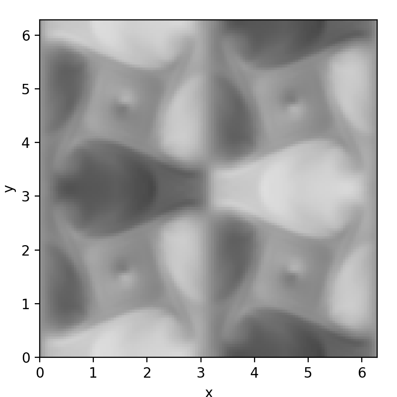
Fig. 26 Output of the plotting code-block based on the 3D TGV example data