dNami syntax
This section introduces the dNami syntax. By using the dNami syntax the user can easily translate differential equations into finite difference code.
Floats
When adding a float to the pseudo-code in an equations.py file, it should be followed by the suffix _wp which makes sure the floating point constant has the correct working precision chosen in the genRhs.py. For example:
F = {'f' : ' 2.0_wp * [f]_1x ' }
In the Python layer, users are encouraged to use the dn.cst() function to ensure consistant floating-point precision across the layers.
Spatial derivatives
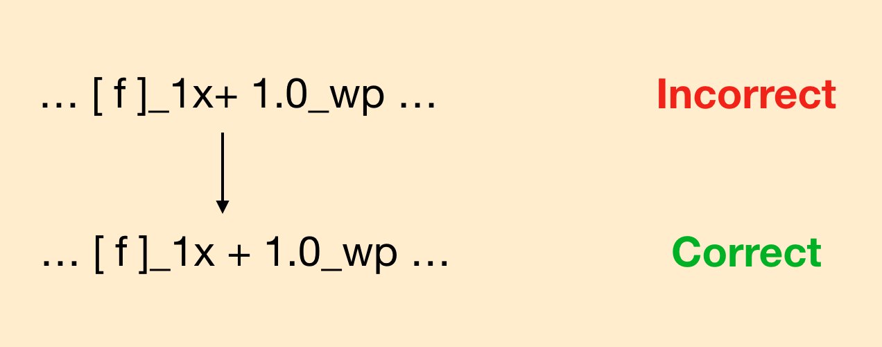
Warning
When specifying derivatives, make sure to leave at least one space after the ‘]_1x’, ‘]_1y’ or ‘]_1z’ notation and the next symbol (this is so that the pseudo-code can be correctly understood and translated). For example:
First order derivative syntax
The tables below show how to express derivatives in the dNami syntax in each of the three spatial directions.
Mathematical notation |
dNami notation |
Description |
|---|---|---|
\[\dfrac{\partial f}{\partial x}\]
|
[ f ]_1x |
First derivative in x direction |
\[\dfrac{\partial f}{\partial y}\]
|
[ f ]_1y |
First derivative in y direction |
\[\dfrac{\partial f}{\partial z}\]
|
[ f ]_1z |
First derivative in z direction |
Second order derivative syntax
To specify second order derivatives, two ways are currently possible. The user can directly specify a second derivative (discretised as a second derivative) or by taking the first derivative twice as detailed below. The two approaches are mathematically equivalent but will yields different results when discretised. The curly-bracket ‘}’ symbol is used when taking a derivative inside another derivative. This approach can also be applied to cross-derivatives.
Mathematical notation |
dNami notation |
Description |
|---|---|---|
\[\dfrac{\partial^2 f}{\partial x^2}\]
|
[ f ]_2xx |
Second derivative in x direction |
\[\dfrac{\partial}{\partial x}\dfrac{\partial f}{\partial x}\]
|
[ {f}_1x ]_1x |
Double first derivative in x direction |
\[\dfrac{\partial}{\partial y}\dfrac{\partial f}{\partial x}\]
|
[ f ]_2xy |
Cross-derivative in x and y directions |
\[\dfrac{\partial}{\partial y}\dfrac{\partial f}{\partial x}\]
|
[ {f}_1x ]_1y |
First derivative in x and y direction |
Higher order derivative syntax
To generate higher-order derivatives, the current stategy involves storing an intermediate derivative and then taking the derivative of that stored variable. This is illustrated in the 1D KdV equations in Quickstart guide where the third order derivative of the field \(u\) is computed by computing and storing the second order derivative and then taking the first derivative of that stored field when specifying the RHS:
varstored = { 'u_xx' : {'symb':' [u]_2xx ','ind':1, 'static': False } }
...
RHS = {'u' : ' epsilon * u * [ u ]_1x + mu * [ u_xx ]_1x ',}